Towards Explainability of Machine Learning Models in Insurance Pricing

Peeking into the black box – an actuarial perspective.

This blog post is a companion piece to the paper of the same title(Kuo and Lupton 2020), which was recently accepted for publication in Variance. In the paper, we discuss details about the need for actuaries to be able to explain machine learning (ML) models. This post provides an accessible summary of the paper and a few code snippets to show how one can get started with model explanation techniques.

Motivation

First, some background: why is it important to be able to explain ML models? There are a few obvious reasons:

1. To comply with relevant Actuarial Standards of Practice or the relevant standards for one’s practicing jurisdiction. There are a lot of standards that pose challenges for “black box” models, so it’s often necessary to have some deep understanding about how a model is working.
2. To communicate results to relevant stakeholders. This may include regulators, colleagues, bosses, auditors, consultants, agents, or even customers. Actuaries don’t operate in a vacuum, so it’s important to make sure you can get the buy-in and support of others.
3. To be a responsible actuary! If you want to use a model, you should have some understanding of what it does and whether or not it is working. The methods we explore here are powerful tools for gaining insight into the effects of your model.

Interpretability

Before we get started, there’s one other question we need to tackle: what does it mean for a model to be interpretable?

The answer really depends on context and audience. Often the inner workings of ML models are not mysterious — the algorithms that generate answers are well-understood, much the same way GLMs are considered to be well-understood. Likewise, it’s worth noting that both GLMs and ML models can pose challenges for interpretation when they become complex.

What qualifies as interpretable, then, really depends on the person asking the questions, the model itself, and the kinds of questions being asked. A seasoned ML or statistics expert will have a very different sense of interpretability than a relative newcomer just by virtue of having deeper understanding of the mechanics of the models in question.

That said, it is possible to sidestep this issue to some extent. The techniques in this paper focus on model-agnostic interpretation strategies. These techniques allow the user to gain a rich understanding of the effects of a model without relying on deep knowledge of the model’s mathematical properties or structure. This broad approach to interpretability allows those unfamiliar with the specific model to gain understanding of how a model is generating predictions and whether those predictions are reasonable.

Questions to Answer

The techniques we introduce here will help to answer three main questions. We pose these questions in the context of ratemaking, though similar questions might be asked in other domains of application. There are many ways to answer these kinds of questions, as we discussed above, but this post will focus on a more limited toolbox of powerful techniques.

The questions and our proposed answers are as follows:

1. What are the most important predictors in the model? Variable importance plots.
2. How do changes to the inputs affect the output on average? Partial dependence plots.
3. For a particular policyholder, which of their characteristics are contributing to the rate they’re being charged (and how much)? Variable attribution plots.

We emphasize that each technique outlined here is not the only way to do things. In fact, they are the simplest starting points with certain drawbacks, and variations and improvements have been built upon them (see the paper for references). You can think of these as the OG approaches.

Examples

Let’s take a look at examples of these Q&As. The working example we consider is a personal auto pure premium model based on actual data from Brazil (more specifically, a neural network, though the model explanation techniques are agnostic with respect to the type of model). For those who would like to follow along with code, check out the GitHub repo.

Permutation Feature Importance

This technique answers the question, “What are the most important predictors in the model?” or, put another way, which predictors are contributing most to the accuracy of predictions?

One way to figure out how much a variable contributes to predictive accuracy would be to compare nested models including and excluding the variable and checking which model performs better on average. However, with complicated models and lots of data, this could be a computationally expensive process. Instead, variable importance plots use a clever workaround: instead of removing a variable entirely and re-fitting, we simply permute the values of the variable, i.e., we randomly rearrange the variable’s values and we see how well the model fits.

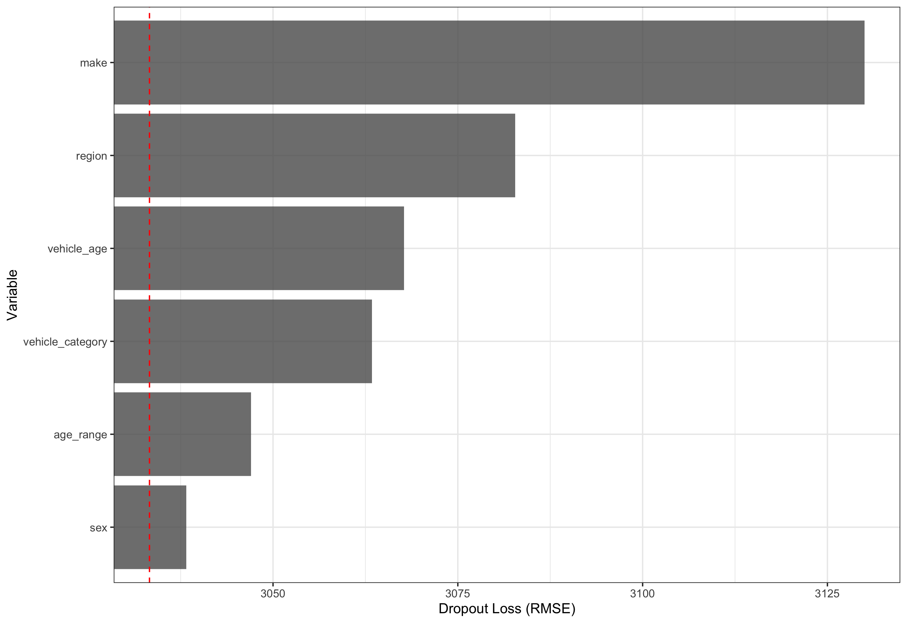
Figure 1: Losses on testing dataset when each predictor’s values are randomly permuted. Red dashed line indicates model without variable permutation.

Here, we see that Make contributes most to the accuracy of the model while Sex contributes the least.

Partial Dependence Plot (PDP)

This technique answers the question, “How do changes to the inputs affect the output on average?”

For highly non-linear models, it could be important to verify that the relationship between a rating variable and pure premium (for instance) makes sense. This technique can be used to review those relationships. This technique works by considering the model’s prediction at a certain level of a variable averaged over all other variables. For example, we might consider the average predicted pure premium at different vehicle ages, averaged over all other modeled variables. This yields a curve reflecting how the pure premium changes on average as the vehicle age changes.

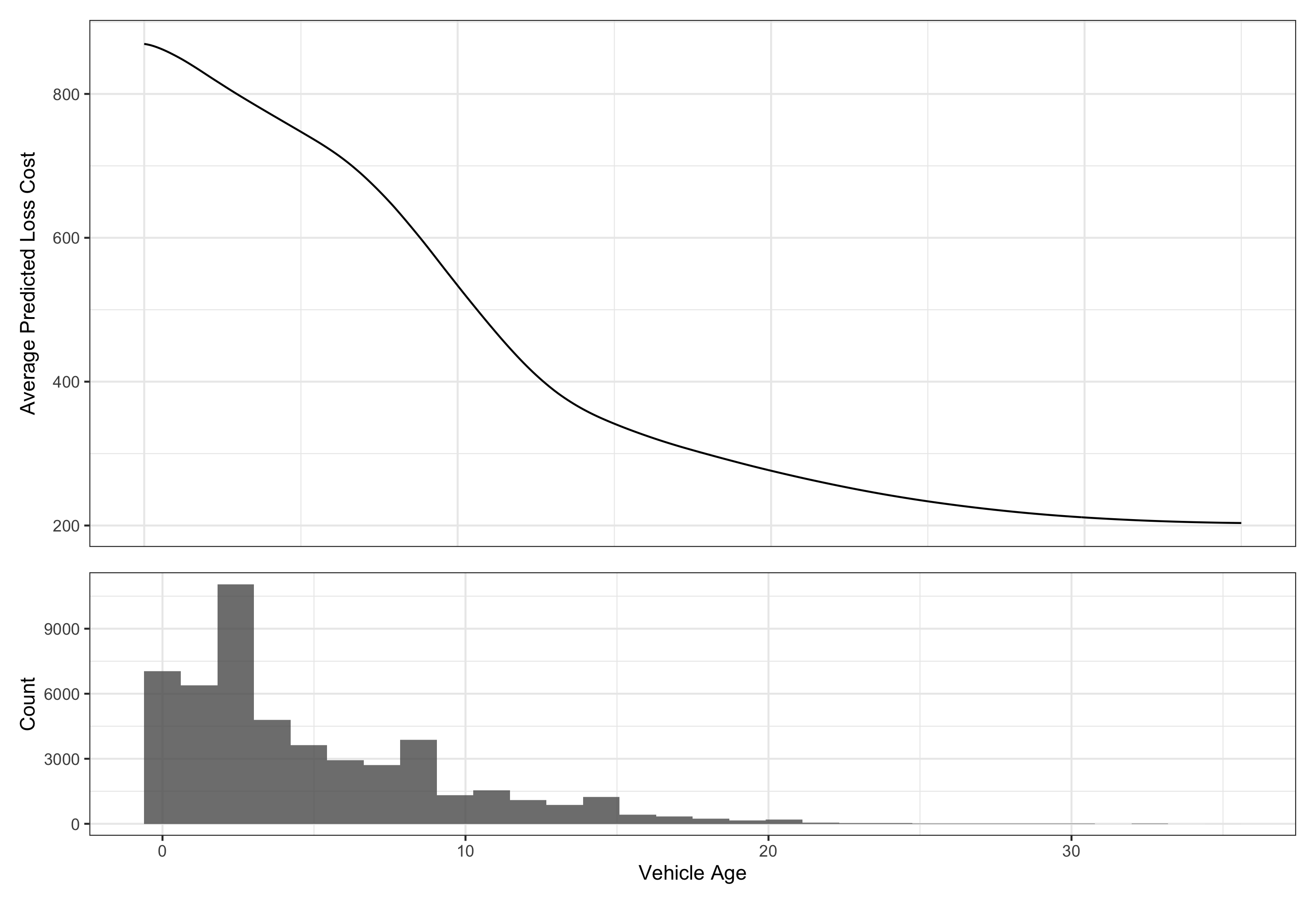
Figure 2: Partial dependence plot and distribution of the Vehicle Age variable.

As the Vehicle Age variable increases, we expect that, on average, our model will predict a lower loss cost. It is appropriate to consider the distribution of the variable when considering its PDP, as sometimes unexpected behavior can appear near values where the variable has thin data.

Variable Attribution

This method answers the common question: what factors most contribute to the rate a policyholder is being charged? For example, a young driver might get a higher auto insurance premium, but the car on the policy might be associated with comparatively low pure premium. How do these factors combine to generate the policyholder’s rate?

This technique can be used to verify that predictions make sense, and it can be used to investigate problematic predictions. Technically, it works by looking at how the model prediction changes as each variable is introduced. So we start with the average prediction (i.e., the model intercept), and then look at how the model changes as each variable is moved from its average, or expected, value to the specific value for a given policyholder.

The verbal description is a little confusing, but it is easy to understand with an example:

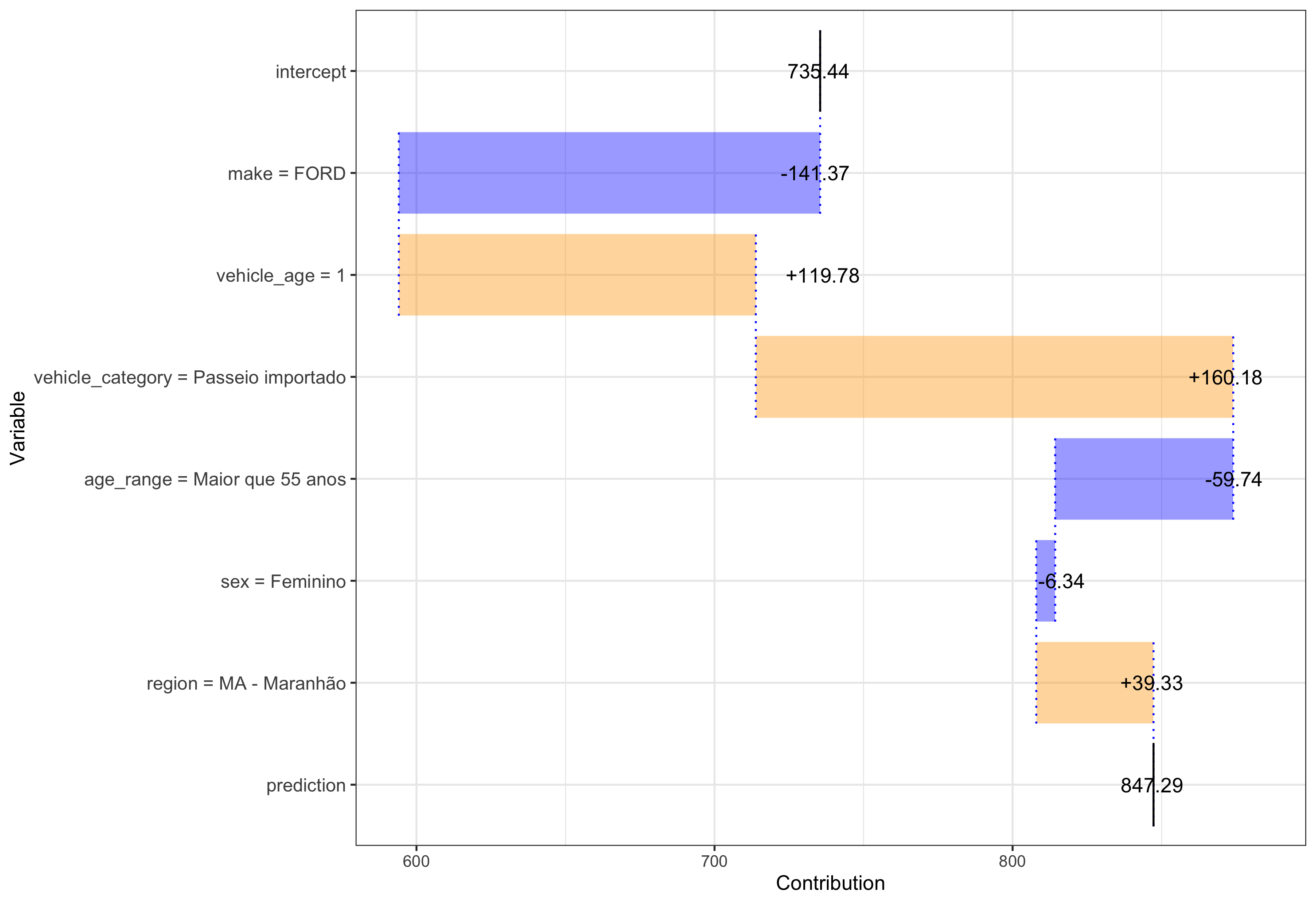
Figure 3: Variable attribution plot for an example policy.

In this case, starting with a model average prediction of R$735 across the entire dataset, our policy has an expected decrease in loss cost of R$141 due to the vehicle being a Ford, an expected increase in loss cost of R$120 due to the vehicle being relatively new (vehicle_age == 1), and so on, until we arrive at the predicted loss cost of R$847.

Conclusion

In this post, we explored three powerful, model-agnostic techniques for understanding, troubleshooting, and communicating model results. It is worth noting that the techniques explored in this post are only one version of a subset of available techniques, and the paper provides references to alternatives.

Finally, we would like to point out a recent tutorial(Lorentzen and Mayer 2020) made available by others, and encourage academics and practitioners alike explore this very interesting topic!